
Methodology
In addition to providing a nationwide representation of historical and current groundwater levels, the project aims to calculate and provide monthly updated short-term groundwater level forecasts (up to 3 months), medium-term groundwater level predictions (up to 10 years) as well as long-term groundwater level projections (up to 2100) for monitoring sites distributed throughout Germany. In a first step, representative monitoring sites in so-called cluster regions were selected from the extensive monitoring site data of the responsible state offices using a nationally uniform method based on Artificial Neural Networks (ANNs). In a second step, groundwater level predictions were calculated at these reference monitoring sites, also using an ANN-based methodology, based on observed and modelled climate grid data from Germany's National Meteorological Service (DWD).
Selection of reference monitoring sites:
In order to select from the pool of monitoring sites provided by the federal states those that can be used as reference monitoring sites and thus for forecasting, a new method was developed that is based on a special type of ANN, the so-called Self-Organising Maps (SOM), and is similar to a classic cluster approach. The aim is to find groups of similar objects, in this case groundwater hydrographs with similar dynamics. To deal with the problem of uneven time series lengths and data gaps, an approach was chosen that describes the dynamics of the hydrographs by so-called features. The features are designed so that they either describe the groundwater dynamics or reveal such a striking property of the time series that corresponding time series can be grouped together.
| Feature-Name | Description |
|---|---|
| Diffsum | Variability, captures the mean magnitude of the slopes, calculated from the median of the sum of the magnitudes of all derivatives |
| Ex Vals | Roughness, high frequency variability |
| Annual Periodicity | Intensity of the annual cycle, calculated by correlating the mean annual periodicity with the complete time series |
| Annual Variance | Variability, periodicity, calculated as median of annual variance |
| Jumps | Inhomogeneities, breaks, partly also variability |
| Longest Recession | Unnaturally long declining groundwater levels, longest sequence without rising values |
| Range Ratio | Superimposed long-period signals |
| Fdif | Variability, captures the frequency of large gradients |
| Skew | Inhomogeneities, outliers, frequent extreme values |
| Standard Error | Measure of dispersion, standardised deviation of the time series |
| Seasonal Behaviour | Time of the maximum in the annual cycle |
| mup / mdown | Rise and fall behaviour, symmetry of hydrograph peaks |
Basically, there are different types of groundwater dynamics that can be described differently with different characteristics. For example, the typical dynamics in a porous aquifer are quite different from those in a karst aquifer, which usually require different characteristics to describe. For this purpose, self-describing mathematical characteristics are extracted from the data, which are then clustered and, in the best case, hydrographs with the same dynamics are assigned to a common cluster. The basic idea in selecting reference monitoring sites is to select a monitoring site whose dynamics are representative for a cluster, i.e. the groundwater dynamics at the other cluster monitoring sites in the area behave similarly to those at the reference monitoring site, so that, for example, predictions of groundwater levels at the reference monitoring site can also be applied to the rest of the cluster.
The reference monitoring site concept, i.e. the reduction of all monitoring stations to a manageable number of reference monitoring stations, is based on the necessary compromise between technical feasibility and the goal of a forecast that is as comprehensive as possible. Only a limited number of sites can be equipped with data loggers and remote data transmission, and the computational effort for the monthly updates must remain manageable.
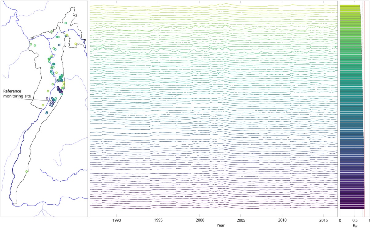
In defining the spatial units to which clustering is applied, the hydrogeological spatial classification of Germany into major districts, regions and sub-regions was chosen (AD-HOC-AG HYDROGEOLOGIE, 2016). A cluster is always located within a major district. In the approach chosen for clustering groundwater hydrographs, however, the spatial location is initially not taken into account. Clustering is performed solely on the basis of the groundwater dynamics of the time series described by the features. Ideally, clusters can be formed that combine monitoring sites that are also spatially close to each other, thus reflecting the groundwater dynamics of a spatially coherent area. However, clusters are also formed by combining hydrographs that behave very similarly but are not spatially close to each other. Depending on the data situation, clusters may also be formed that group hydrographs that behave very specifically and do not resemble any other hydrograph. The latter clusters are in principle not suitable for either the selection of reference monitoring sites or the subsequent prediction of groundwater monitoring sites and are usually discarded. For the other two cluster types, it can be assumed that the monitoring points or hydrographs within the cluster behave in a similar way, and therefore it makes sense to select a reference monitoring site that can later be used to predict the other points in the cluster (regardless of their spatial location).
The cluster centre is formed by the hydrograph whose descriptive characteristics are considered most representative of all other hydrographs in the cluster. As the distance from the cluster centre increases, the similarity to the cluster centre usually decreases. As the clustering is based on the similarity of the descriptive features of the hydrographs, but for the later prediction a similarity of the hydrographs with respect to their actual values is relevant, the distance to the cluster centre is only conditionally suitable for the selection of the reference measurement point. Since a correlation analysis within the formed clusters showed that the measurement points close to the cluster centre are not necessarily the most highly correlated with all other measurement points of the cluster, each hydrograph was correlated with every other hydrograph for the reference measurement point selection of a cluster. The average of the weighted correlation coefficients Rw was calculated for each hydrograph and the hydrographs were sorted by descending Rw. The (new) cluster centre is thus the monitoring station that correlates best with all others on average.
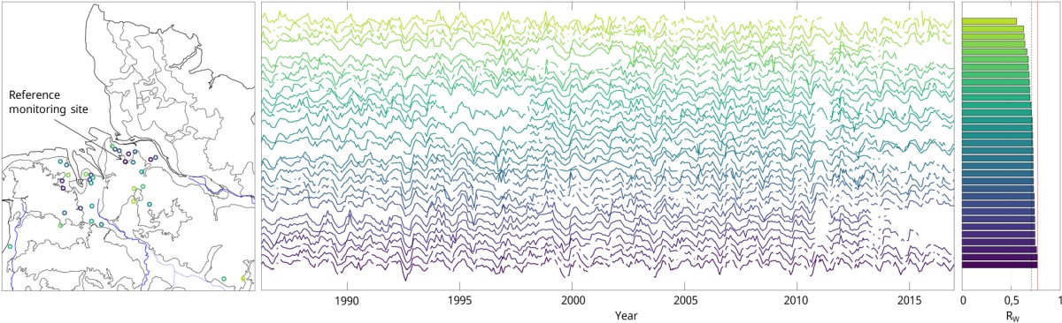
Even for relatively homogeneous clusters, the correlation with the rest of the cluster's hydrographs drops sharply for hydrographs at the edge of the cluster. As these monitoring sites are not suitable for prediction, they are removed by truncating the cluster towards the edge above a certain threshold Rw. For most clusters, a threshold of 0.5 to 0.6 has been found to be appropriate. After truncating the cluster, the mean of the weighted correlation coefficients for the remaining sites is recalculated and the hydrographs are again sorted according to descending Rw. This essentially results in a purified homogeneity of the cluster.
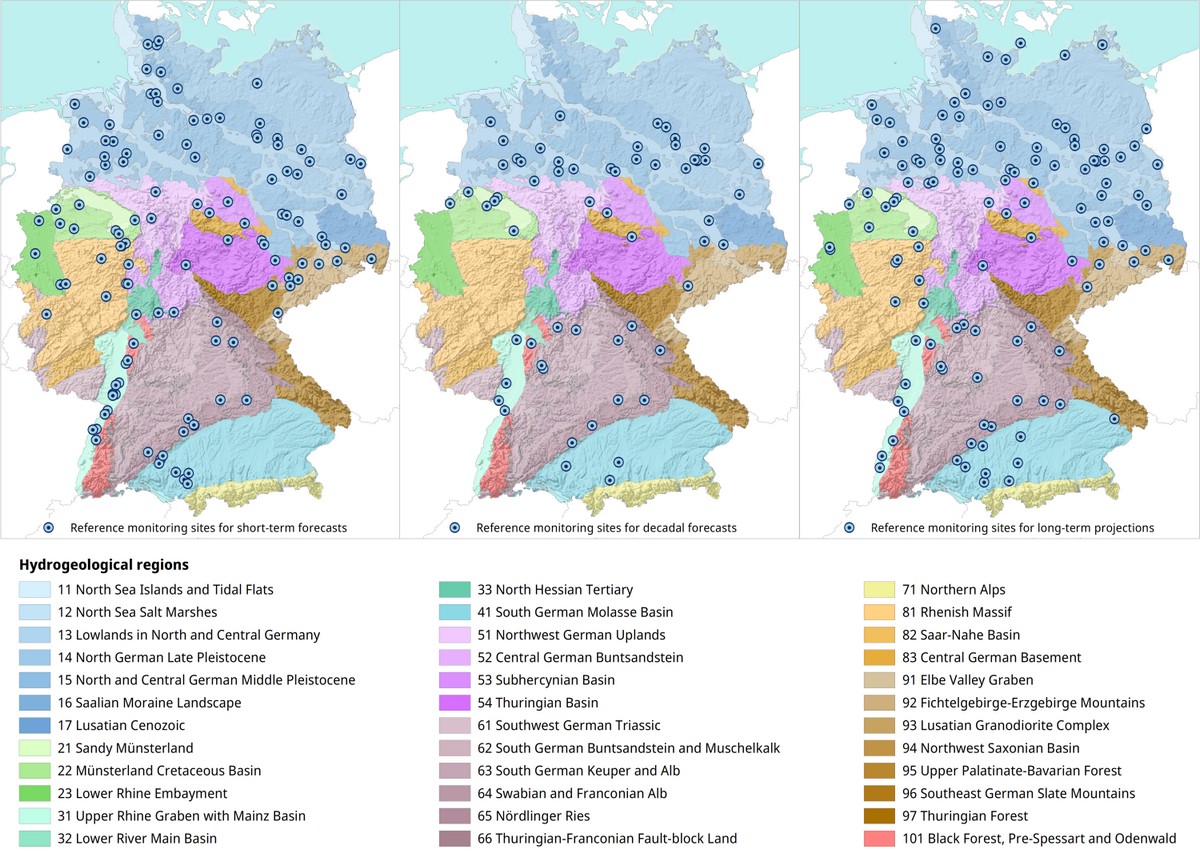
After testing and optimising the method in the hydrogeological district 3 (Upper Rhine Graben with Mainz Basin and North Hessian Tertiary), the method was applied to the entire dataset. After pre-processing, limitation of the investigation periods, sorting out due to inhomogeneities and revision due to the change of the forecast approach, 4392 monitoring sites in about 120 clusters remained, which were classified as potentially suitable for a short-term forecast on the basis of the reference monitoring site of the respective cluster (monitoring site with the highest correlation to all other monitoring sites in the cluster).
Due to the particular challenges of long-term forecasting, the results of which cannot be validated, not all defined reference monitoring sites could be used for the medium-term prediction and the long-term projection. Instead, for each forecast horizon, a seperate set of monitoring sites was defined based on all reference and cluster monitoring sites. For reasons of data availability, model quality and plausibility, 60 groundwater monitoring sites remained suitable for the medium-term decadal forecast and 118 groundwater monitoring sites for the long-term projection to 2100. The number of monitoring sites for the medium-term and long-term projection is therefore only partly the same as for the short-term forecast.
The method developed is very suitable for defining the reference monitoring sites themselves and the sites to which they serve as a reference. It offers a number of advantages over previously used methods. It provides a mathematical measure of the quality of the connection between reference and prediction sites. It standardises and mathematically objectifies the selection, which has often been subjective and varied from state to state. It also opens up the possibility of recognising relationships in the data that were previously not possible due to the sheer volume of data.
The representation of the remaining monitoring sites for the short-term forecast shows in some cases a very good spatial coverage. However, in other areas the density of the remaining monitoring sites is low, especially where the coverage was already rather low to begin with. This is probably due firstly to the hydrogeological conditions, which cause the groundwater hydrographs to behave very differently locally, making it difficult to form meaningful clusters (e.g. in the Pre-Alps in the area of the Molasse Basin), and secondly to a lack of data quality. In particular, incomplete data and short measurement periods make clustering and subsequent forecasing difficult.
Prediction of groundwater levels at reference monitoring sites:
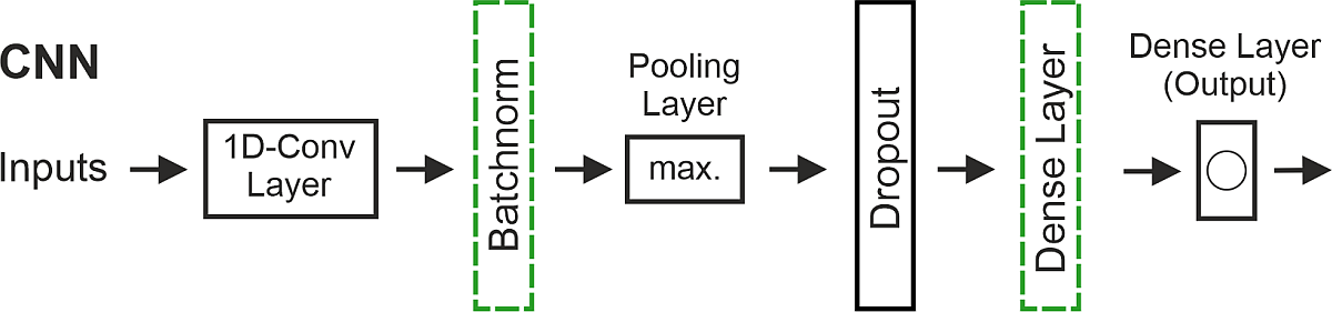
The use of algorithms to predict groundwater levels is also based on the Artificial Neural Network (ANN) method. In recent years, numerous studies have shown that CNN (Convolutional Neural Network), LSTM (Long Short-Term Memory) and NARX (Nonlinear Auto-Regressive eXogenous input) models are very suitable for predicting groundwater levels (Wunsch et al., 2021). Only one-dimensional Convolutional Neural Networks (CNNs) are used to predict groundwater levels on the national scale.
One-dimensional Convolutional Neural Networks (CNNs) are a special type of ANN. They are well suited to Machine Learning (ML) and Artificial Intelligence (AI) applications in the fields of image and speech recognition. CNNs usually consist of at least three different layers. Convolutional layers, the first type, usually consist of a large number of filters and feature maps. Each filter has a fixed size; its input is also called the receptive field. Step by step, all the filters are moved over the input data, creating a feature map specific to each filter, i.e. each filter extracts different, specific features from the data. Convolutional layers are usually followed by pooling layers, which downsample the feature map of the previous layer, i.e. the information is consolidated by applying simple operations such as averaging or maximum selection to subsections of the data. Similar to LSTM models, multiple convolutional and pooling layers can be stacked in different orders. The last layer is then followed by a dense layer with one or more output neurons.
Hydrometeorological grid data (HYRAS) provided by the DWD were used as input for the training. The data contain daily observations of precipitation (P) and temperature (T) from 1951 to 2015, with a resolution of 12.5 × 12.5 km. Different versions of the data are available, resulting in different end dates for the available time series. P v2.1 and T v2.0 were used for the long-term forecast models. These data end at the turn of the year 2015/16. The decadal predictions start in 2022, so more recent climate data were needed up to and including 2021. Therefore, the newer versions of precipitation (P) v3.0, temperature (T) v4.0 and relative humidity (RH) v4.0 were used. P v3.0 is continuously updated and made available online, but temperature, like the previous versions, currently ends in 2015. The resulting gap until 2022 was filled with data from E-OBS v25.0e (Copernicus Climate Change Service C3s). This is a European dataset of gridded and regionalised climate observations. Once available, E-OBS data will be replaced by HYRAS data.
Hindcasts from the DWD were used to evaluate the precision of the groundwater level forecasts, due to the absence of operational observations. Hindcasts, also known as backward forecasts, are forecasts that start in the past and are compared with observations to assess the quality of the forecasts. The empirical-statistical downscaling method EPISODES, developed by the DWD, was used to generate the grid dataset. The method is based on seasonal forecasts from the German Climate Forecast System (GCFS). Model-based recalculations of daily precipitation and temperature data with a resolution of 12.5 × 12.5 km are available for the years 1990 to 2017.
| Short-term forecasts (1 week, 1 month, 3 months) | Decadal predictions (2022 - 2031) | Long-term projections (up to 2100) |
|
|---|---|---|---|
| Training | DWD-HYRAS data | DWD-HYRAS data | DWD-HYRAS data |
| Evaluation | DWD-HYRAS / ERA5-Land data plus EPISODES-Hindcasts of the DWD | DWD-HYRAS | DWD-HYRAS data |
| Operational forecast | EPISODES data of the DWD | Ensemble data of the MPI-ESM-LR | DWD Core Ensemble RCP scenarios 2.6, 4.5 and 8.5 |
Data from the Max Planck Institute for Meteorology's Low Resolution Earth System Model (MPI-ESM-LR) were used as the basis for the decadal predictions. These have been processed using the EPISODES method and are available at a geographical resolution of 5 km and bias-adjusted to observational data. The data are also available as ensemble simulations in 16 different model runs. The simulation starts in 2021 and the prediction period covers the years 2022 to 2031.
In the case of the long-term projections, the DWD core ensemble models were used to generate the input data. The three RCP scenarios 2.6, 4.5 and 8.5, which according to the Intergovernmental Panel on Climate Change are representative concentration paths for describing scenarios for the development of absolute greenhouse gas concentrations in the atmosphere, were examined. The assessment was carried out using linear trend analysis of annual means and analysis of changes between the start of the simulation in 2014 and the end of the simulation in 2100 (Wunsch et al., 2022).
Literature:
AD-HOC-AG HYDROGEOLOGIE (2016): Regionale Hydrogeologie von Deutschland – Die Grundwasserleiter: Verbreitung, Gesteine, Lagerungsverhältnisse,
Schutz und Bedeutung. – Geol. Jb., A 163: 456 pp., 264 fig.; Hanover.
KREIENKAMP, F., PAXIAN, A., FRÜH, B. et al. (2019): Evaluation of the empirical–statistical downscaling method EPISODES. – Clim Dyn 52, 991–1026. DOI: 10.1007/s00382-018-4276-2.
OHMER, M., LIESCH, T., HABBEL, B., HEUDORFER, B., GOMEZ, M., CLOS, P., NÖLSCHER, M. & BRODA, S. (2026): GEMS-GER: a machine learning benchmark dataset of long-term groundwater levels in Germany with meteorological forcings and site-specific environmental features. – Earth System Science Data, 18, pp. 77–95. DOI: 10.5194/essd-18-77-2026.
WETZEL, M. et al. (2026): Bundesweite Entwicklung der Grundwasserstände seit 1991: Langzeittrends, Variabilität und Auswirkungen der jüngsten Trockenphase. – Grundwasser – Zeitschrift der Fachsektion Hydrogeologie. DOI: 10.1007/s00767-026-00616-4.
WUNSCH, A. & LIESCH, T. (2022): Anwendung neuer Vorhersageprodukte. – Zwischenbericht Arbeitspaket 3, 39 pp., 22 fig., 4 tab.; KIT, Karlsruhe.
WUNSCH, A. & LIESCH, T. (2021): Entwicklung, Anwendung und Evaluierung von Deep Learning Ansätzen zur Grundwasserstandsvorhersage.
– Zwischenbericht Arbeitspaket 1, 83 pp., 24 fig., 1 tab., 4 Ann.; KIT, Karlsruhe.
WUNSCH, A. & LIESCH, T. (2020): Entwicklung und Anwendung von Algorithmen zur Berechnung von Grundwasserständen an Referenzmessstellen auf Basis der Methode Künstlicher Neuronaler Netze. – Abschlussbericht Projektphase I, 183 pp., 61 fig., 11 tab., 13 ann.; KIT, Karlsruhe. DOI: 10.5445/IR/1000136522.
WUNSCH, A., LIESCH, T., BRODA, S. (2022): Deep learning shows declining groundwater levels in Germany until 2100 due to climate change. – Nat
Commun 13(1), 1221. DOI: 10.1038/s41467-022-28770-2.
WUNSCH, A., LIESCH, T. & BRODA, S. (2022): Feature-based Groundwater Hydrograph Clustering Using Unsupervised Self-Organizing Map-Ensembles. – Water Resour. Manage., 36(1): 39–54. DOI: 10.1007/sll269-021-03006-y.
WUNSCH, A., LIESCH, T., BRODA, S. (2021): Groundwater level forecasting with artificial neural networks: A comparison of long shortterm memory
(LSTM), convolutional neural networks (CNNs), and non-linear autoregressive networks with exogenous input (NARX). – Hydrol. Earth Syst.
Sci. 25 (3), pp. 1671–1687. DOI: 10.5194/hess-25-1671-2021.