Groundwater level forecasts predict what the groundwater level will be at a specific location at a specific time. Forecasts are based on current groundwater levels, past groundwater levels and expected precipitation and temperatures for a future period. The forecasts are produced using mathematical models, in this case a data-driven statistical prediction model using artificial neural networks and machine learning, and can be used to warn of possible high or low water levels and thus plan water management measures.
Groundwater level forecasts can be an important tool for sustainable groundwater management. In agriculture, they can be used to provide early warning of declining groundwater resources in order to optimise irrigation and reduce water consumption. They can also be used in the construction or planning of infrastructure projects to minimise the risk of flooding and damage to buildings, roads and bridges. Groundwater level forecasts can also raise public awareness of potential droughts due to low groundwater levels and overflow situations due to high groundwater levels.
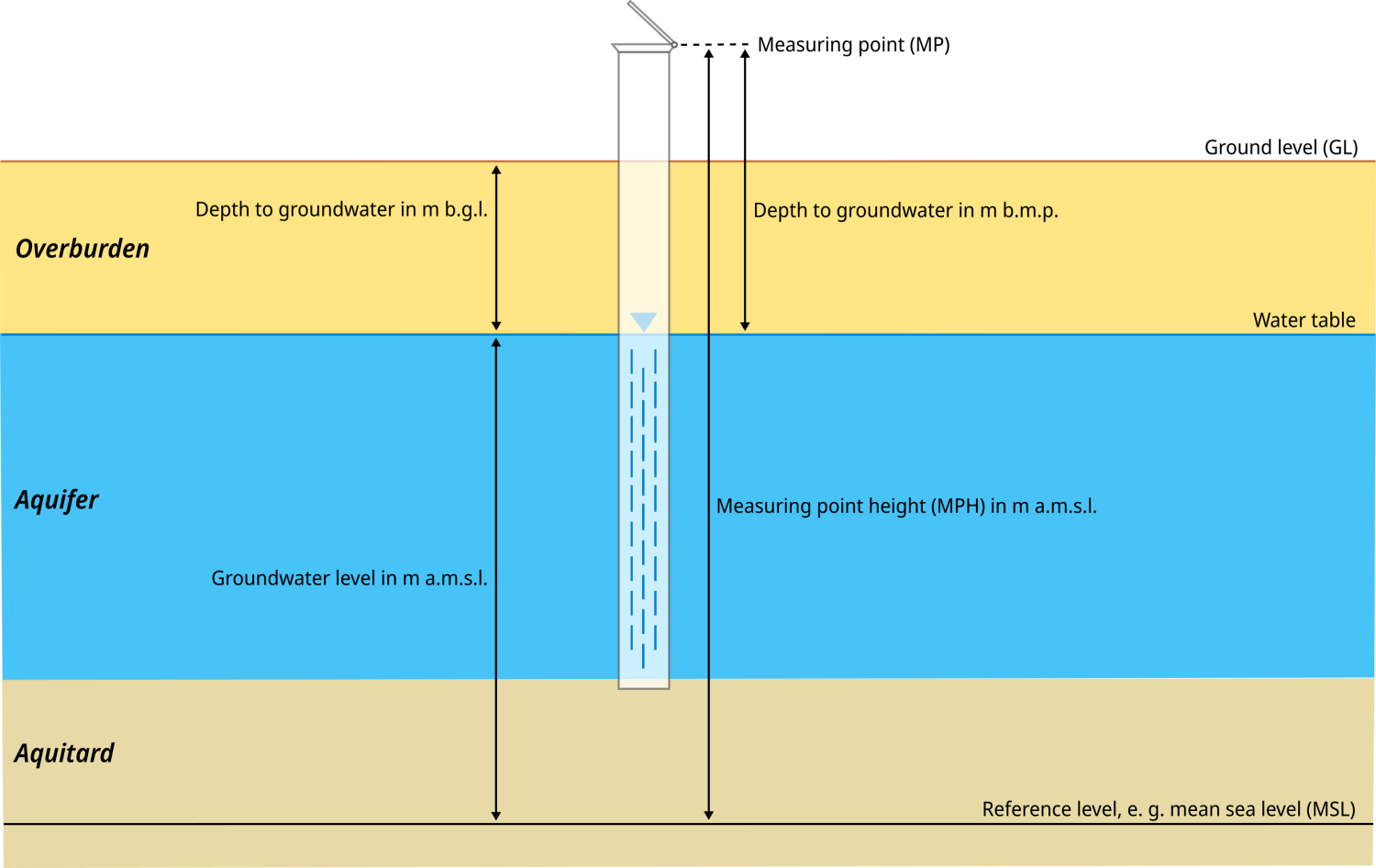
According to DIN 4049-3, the groundwater level is the height of the groundwater table above or below a horizontal reference level, usually above mean sea level or below ground level. Colloquially, the terms groundwater level and groundwater table are often used interchangeably. The groundwater table is defined as the pressure-balanced interface between the groundwater and the atmosphere.
The groundwater level at a well or monitoring site can be expressed in metres above sea level (m a.s.l.), metres below ground level (m b.g.l.) or metres below the level of the monitoring point (m b.m.p.).
Schematic illustration of a groundwater monitoring site and common groundwater levels measured. Source: BGR
If the groundwater level at a monitoring site is measured over a long period of time, the result can be presented graphically in the form of a groundwater level hydrograph. The groundwater level can be shown on maps as point information or in the form of a groundwater contours (also called groundwater isohypses). The groundwater level can be shown on a specific date, as an average over a defined period of time or as a range of fluctuations over a specific period of time.
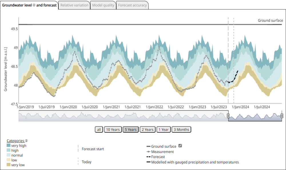
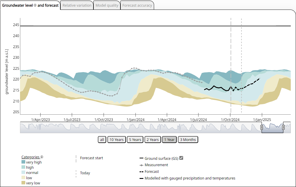
Groundwater level hydrograph of a monitoring site over a period of 5 years and forecast for 3 months. In order to classify the groundwater levels, all mean weekly groundwater levels from the 30-year reference period 1991 - 2020 are divided into five classes and shown in graded colours as a background. "Very low" means < 10% of all values, "low" between 10 and 25% of all values, "normal" between 25 and 75% of all values, "high" between 75 and 90% of all values and "very high" > 90% of all values for the respective calendar week from 1991 - 2020. Source: BGR
Monitoring of groundwater levels is important to identify problematic changes in a timely manner and, if necessary, to take countermeasures to prevent negative impacts on or caused by groundwater resources. A fall in the water level can cause damage to vegetation and damage to buildings due to subsidence. A rise in groundwater levels can also cause damage to structures or, in extreme cases, render agricultural land unusable.
Groundwater levels can be measured in (not pumped) drilled wells, piezometers, uncased hardrock boreholes and dug wells or natural pits. Ideally, it is measured in a specially constructed monitoring well. Traditionally, groundwater levels have been measured manually using an electric contact meter.
Nowadays, the most common type of monitoring station is an automated one, where the groundwater level is continuously measured by a pressure sensor and stored in a data logger, which is visited and read by local staff at regular intervals. There is often the possibility of remote data transmission and the data can be transmitted to the relevant authority via the mobile phone network and displayed in real time.
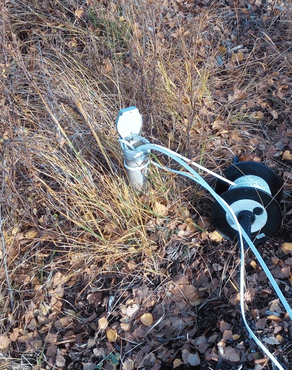
Measuring the groundwater level using an electric contact meter during groundwater sampling. Source: BGR
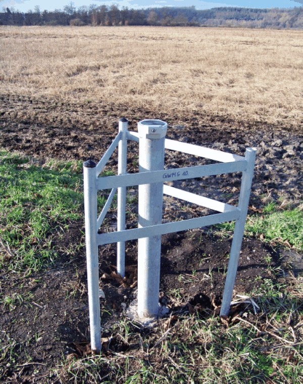
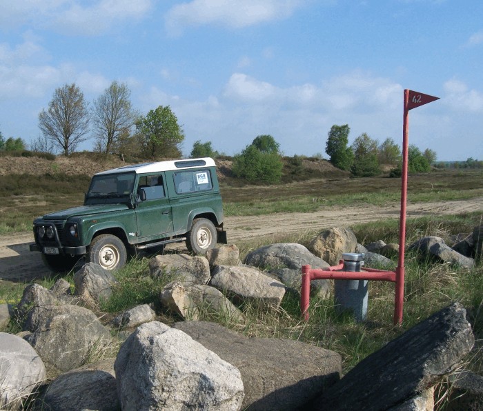
Groundwater monitoring site in the Seeländereien. To protect against vandalism, all components (including GPRS dial-up functionality) are located under a standard level cap. Source: BGR
In order to measure natural and as unaffected groundwater levels as possible, monitoring sites should be selected where the groundwater surface is not, or as little as possible, influenced by groundwater abstraction such as waterworks or agricultural irrigation wells.
The groundwater level in an aquifer is controlled by the relationship between recharge, storage and discharge. Physical properties such as the porosity, permeability and thickness of the rocks that make up the aquifer influence this system. So do climatic and hydrological factors such as the timing and amount of recharge from precipitation, subsurface runoff to surface water and evapotranspiration. When the rate of recharge to an aquifer exceeds the rate of discharge, the water table rises. Conversely, if groundwater abstraction or discharge is greater than groundwater recharge, the groundwater stored in the aquifer is used up and water levels fall.
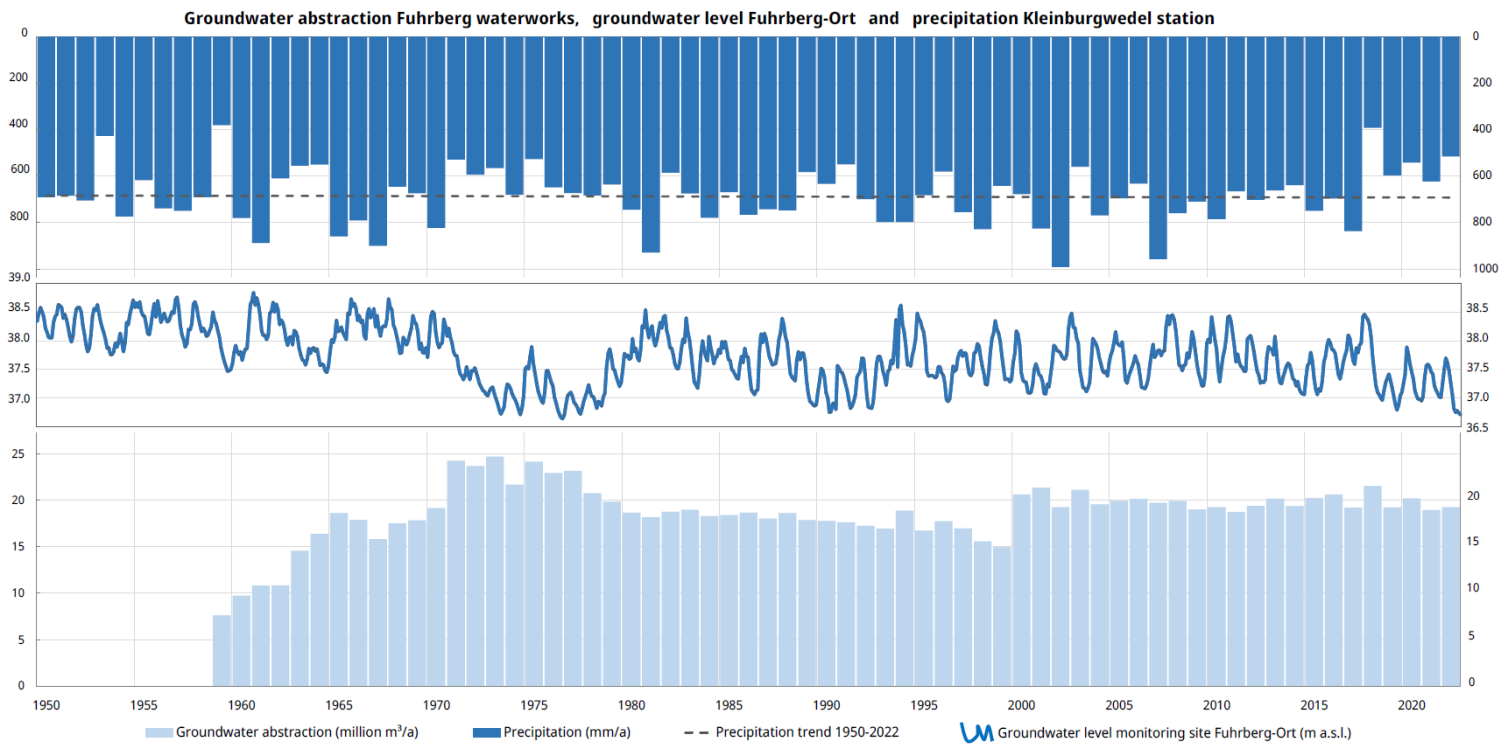
Water levels in many aquifers in Germany follow a natural seasonal pattern. They typically rise in winter and spring due to higher precipitation and groundwater recharge, and fall in summer and autumn due to lower recharge and higher evapotranspiration. The magnitude of water level fluctuations can vary greatly from season to season or year to year, depending on climatic conditions. Seasonal fluctuations are amplified in the catchment areas of waterworks and irrigation wells, where more groundwater is abstracted in summer than in winter, and as a rule, no groundwater is abstracted from the latter in winter.
Example of groundwater levels at the Fuhrberg-Ort monitoring site with a typical annual cycle (middle), depending on annual precipitation (top) and annual production rates of the Fuhrberg waterworks (bottom). Data: DWD, NLWKN & Region Hannover. Source: BGR
Natural, climate-related fluctuations in groundwater levels are overshadowed by the effects of human activities. For example, increased surface sealing, deforestation and drainage of wetlands can accelerate surface runoff and reduce groundwater recharge. Conversely, agricultural tillage, damming of streams, climate-adapted forest conversion and the creation of artificial wetlands can increase groundwater recharge. Long-term and comprehensive monitoring of water levels is a prerequisite for obtaining relevant and reliable results and thus contributing to groundwater protection.
Groundwater monitoring site
Groundwater monitoring sites are mainly used to observe groundwater levels and flow conditions, to take samples for groundwater quality assessment and to determine the hydraulic properties of the aquifer. They are also known as 'observation' or 'monitoring' wells, or simply as water level gauges, monitoring tubes or piezometers.
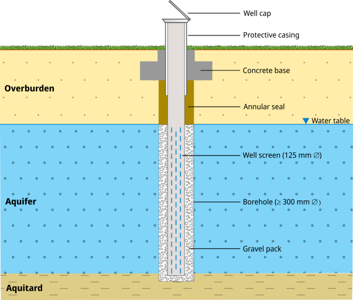
A monitoring well usually consists of PVC pipes of 5 - 15 cm in diameter, whicht are screwed together to form a watertight seal. The pipes are placed in the centre of a previously drilled borehole using spacers. To protect against accidental or deliberate damage, the top of the monitoring well, the monitoring head, should be terminated, where possible, with a steel pipe and a securely lockable well cap. The steel tube should be securely anchored in a concrete foundation. If the monitoring point has an above-ground termination, it should be provided with collision protection and a level flag to make it visible in the terrain. The lower part of the monitoring well usually consists of a well screen, which is installed in the area of the groundwater-filled part of the aquifer. The annular space around the screen is filled with filter gravel and the annular space above is sealed with clay or a clay-cement mixture to prevent infiltration of water from the surface.
Schematic structure of a groundwater monitoring site (left), Source: BGR and groundwater monitoring site in the Colbitz-Letzlinger Heide (right), Source: BGR.
Groundwater monitoring wells, like other types of wells, can provide access to poor quality water, pollutants and contaminants. As monitoring wells are often deliberately located in areas affected by pollution, they pose a particular threat to groundwater quality if they are not properly constructed, maintained and dismantled. For this reason, their construction is subject to specific rules, such as those set out in DVGW Code of Practice W 121 "Construction and Extension of Groundwater Monitoring Stations" or in the leaflet "Construction of Groundwater Monitoring Stations" of the Groundwater Monitoring Working Group.
In the groundwater level prediction method used here, a reference monitoring site is a site whose dynamics are representative of an area or cluster. This means that the dynamics of the groundwater hydrograph at other monitoring sites in the cluster are similar to those at the reference monitoring site, so that, for example, predictions of groundwater levels at the reference monitoring site can also be applied to the rest of the cluster.However, this does not mean that the groundwater level in metres above sea level at the cluster monitoring sites will be the same as at the reference monitoring site.
For this purpose, the groundwater level time series were described with a maximum of 12 different characteristics and self-describing mathematical parameters were extracted from the data, which were then grouped (clustered) and groundwater hydrographs with the same dynamics were assigned to a common cluster.
The hydrographs were then correlated with each other for each cluster, the mean of the weighted correlation coefficient Rw was calculated for each hydrograph and finally the hydrographs were sorted according to decreasing Rw. The reference monitoring site is generally the monitoring site which shows the highest agreement with the dynamics of the groundwater hydrographs compared to all other monitoring sites in the cluster, or which correlates best on average with all other monitoring sites in the cluster and at the same time shows very good predictability.
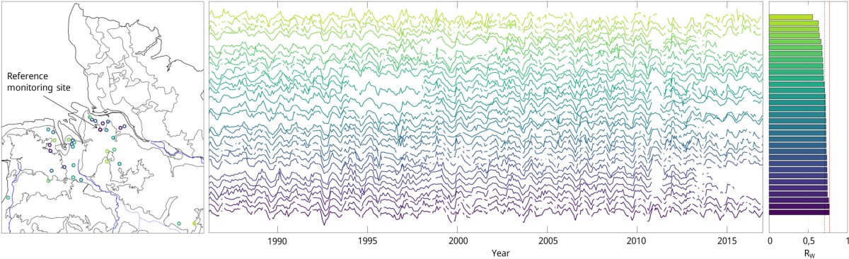
Map of cluster 37 in the major hydrogeological district 1 (North and Central German unconsolidated rock region) with the location of the reference monitoring site (left) and stacked z-transformed hydrographs of the corresponding cluster monitoring sites (middle). The colouring and stacked order reflect the weighted intra-cluster correlation Rw, also shown as a bar chart (right). The average correlation Rw is 0.71, the highest correlation Rw is 0.77 (lowest groundwater hydrograph). Source: BGR & KIT
The reference monitoring site concept, i.e. the reduction of all groundwater monitoring wells to a manageable number of reference monitoring sites, is based on the necessary compromise between technical feasibility and the goal of a prediction that is as comprehensive as possible. Only a limited number of monitoring sites can be equipped with data loggers and remote data transmission, and the computational effort for the monthly updates must remain manageable.
Cluster monitoring sites are a group of monitoring sites that are representative of an area or cluster in AI-based groundwater level prediction, usually defined by spatial proximity and/or a similar hydrogeological situation. Cluster monitoring sites in a cluster are similar in the dynamics of their groundwater hydrographs.
The cluster monitoring point with a very high correlation coefficient Rw and at the same time very good predictability within a cluster is usually the reference monitoring site.
Climate
Climate models are complex mathematical models that simulate the Earth's climate system in the past and calculate possible climate scenarios for the future. They represent reality in a simplified way and can only approximate the climate system with its various physical and chemical processes. Climate models therefore do not provide climate predictions, but only climate projections. This means that they provide information on how the climate will change under the conditions included in the model, i.e. what will happen if people behave as described in the scenario.
Climate models contain various components such as an atmosphere and ocean model, as well as other components such as an ice, snow and vegetation model. Each climate model consists of a 3-dimensional grid that covers the entire globe. A large number of parameters are calculated for the many grid points. Climate models are the most complex and computationally intensive models available today.
A distinction is made between global climate models (GCMs) and regional climate models (RCMs). Global climate models cover the entire troposphere and have a very coarse resolution of about 100 x 100 kilometres, while regional models represent the same model physics only for a specific geographical section of the Earth with a fine resolution of up to 5 x 5 kilometres. For Germany, a DWD core ensemble (version 2018) with five or six global and five or six regional climate models is available for the three RCP scenarios 2.6, 4.5 and 8.5.
The DWD core ensemble is regularly revised to incorporate new climate projections.
Climate scenarios, also known as climate change scenarios, are assumptions about the likely evolution of human influence on the Earth's climate system and its components such as temperature, precipitation and wind. In recent years, science has developed a wide range of possible scenarios that describe the human impact on the climate.
These scenarios are also known in the scientific community as Representative Concentration Pathways (RCPs). The scenarios describe possible futures for the global economy and associated greenhouse gas emissions. They are used to examine the environmental and social impacts of climate change and were developed for the Intergovernmental Panel on Climate Change's (IPCC) 5th Assessment Report (see RCP scenarios).
RCPs - Representative Concentration Pathways are scenarios that include time series of emissions and concentrations of all greenhouse gases, aerosols and chemically active gases, as well as land use and land cover. The word 'representative' means that each RCP represents only one of many possible scenarios that would result in the specific radiative forcing characteristics. The term 'path' emphasises that it is not only the long-term concentration values that are of interest, but also the time course that leads to that outcome.
RCPs usually refer to the part of the concentration path that extends to the year 2100 and for which the integrated assessment models have produced emissions scenarios. Each scenario describes a possible future and the associated greenhouse gas emissions.
In the fifth report of the Intergovernmental Panel on Climate Change (IPCC), four RCPs were selected from the published literature and used as the basis for climate predictions and projections:
RCP scenario 2.6 represents a path where radiative forcing peaks at around 3 W/m2 before 2100 and then declines. Greenhouse gas emissions would not exceed 490 parts per million (ppm) and global warming would likely be limited to below 2°C above pre-industrial temperatures.
RCP scenarios 4.5 and 6.0 describe two intermediate stabilisation pathways, where the radiative forcing after 2100 is around 4.5 W/m2 and 6.0 W/m2, respectively. Greenhouse gas emissions would increase to about 650 ppm and 850 ppm by 2100.
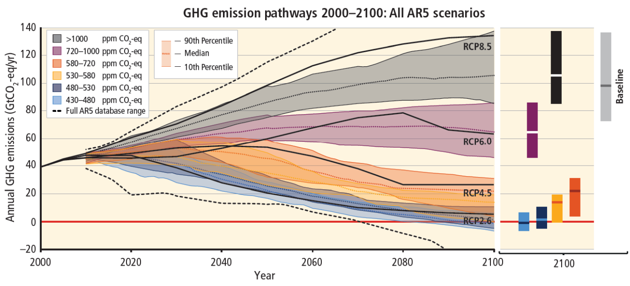
RCP scenario 8.5 is a high path where radiative forcing reaches more than 8.5 W/m2 in 2100 and remains high until 2300. Greenhouse gas emissions reach more than 1370 ppm in 2100. This scenario is also referred to as the 'business-as-usual scenario'.
Global greenhouse gas emissions (gigatonnes of CO2 equivalent per year, Gt CO2 eq/a) in baseline and mitigation scenarios for different long-term concentration levels. Source: IPCC 2014 Literature:
IPCC (2014): Climate Change 2014: Synthesis Report. Contribution of Working Groups I, II and III to the Fifth Assessment Report of the
Intergovernmental Panel on Climate Change [Core Writing Team, R.K. Pachauri and L.A. Meyer (eds.)]. IPCC, Geneva, Switzerland, 151 pp.
Measure of quality
Model quality is an important concept in modelling. Modelling is about finding a mathematical approximation for the relationship between influencing factors and measured values (target variable) so that, for example, predictions can be made for this target variable. Once such a model has been determined, it is important to know how well the model actually works, or how well the predictions match the actual measured or observed values. This is called model quality.
The prerequisite for determining the quality of the model is the partitioning of the data set available for modelling. The data set is first divided into a training period and a test period. The ratio of these two parts is typically 80% to 20%, but can vary depending on the application and the amount of data. In our application, the last 3 years of the measured time series are used as the test period, while the training period is at least 10 years. The model quality is then determined for the test period. There are many methods and measures to numerically determine model quality, such as Mean Absolute Error (MAE), Nash-Sutcliffe Efficiency (NSE) or Root Mean Squared Error (RMSE). Each of these measures has different advantages and disadvantages, which is why several are often calculated at the same time. The numerical determination is important for comparing models and finding the best possible model.
Like model quality, forecast accuracy is a critical factor in evaluating a model. Forecast quality describes how well a model can predict future data. Different methods or error criteria can be used to determine prediction quality. The bias, the correlation, the Kling-Gupta Efficiency (KGE), the Nash-Sutcliffe Efficiency (NSE), the Persistency Index (PI), the Root Mean Squared Error (RMSE) and R-squared (R2) are used and calculated to assess the prediction accuracy of the models used to forecast groundwater levels. These statistical measures are described below.
Each error criterion has advantages and disadvantages and considers different aspects of prediction quality; none of them alone allows a comprehensive assessment. For this reason, several error criteria should always be calculated simultaneously and used for evaluation.
The bias describes systematic deviations between the predictions of a model and the actual values; it reflects the average error of a prediction. Bias values range from \(-\infty\) to \(\infty\). A positive bias means that the model tends to overestimate values, while a negative bias means that it tends to underestimate values. A bias value of 0 would indicate a perfect model.
The bias is calculated using the following formula, where \(o_i\) is the observed values, \(p_i\) is the predicted values and \(n\) is the number of predicted values.
\[Bias=\frac 1n{\sum_{i=1}^{n}(o_i-p_i)}\]
It is important to note that bias should be considered along with other metrics such as Root Mean Squared Error (RMSE) or R-squared (R2) to provide a comprehensive picture of a model's performance.
Correlation is a measure of how closely two variables are related, or whether there is a clear link.
Correlation is often measured by the correlation coefficient R (also known as Pearson's correlation or linear correlation), which can take values between -1 and 1. A value of 1 means that the relationship is perfectly positive, i.e. the two variables always move together in the same direction. When one variable increases, the other also increases and vice versa. A value of -1 indicates a perfect negative relationship, i.e. the two variables always move in opposite directions. A value of 0 means that there is no linear relationship between the variables.
The correlation coefficient R is calculated as follows::
Here \(o_i\) stands for the observed values, \(\bar o\) for their mean, \(p_i\) for the predicted values, \(\bar p\) for their mean and \(n\) for the number of observations.
It is important to note that correlation only measures the linear relationship between variables. The absence of a linear relationship does not mean that other types of relationship do not exist, such as quadratic or exponential.
Kling-Gupta Efficiency (KGE) is a measure of the predictive accuracy of hydrological models. It helps to understand how well a model predicts outcomes.
The KGE metric considers three important aspects: agreement in terms of mean, agreement on the variability, and agreement on the correlation between the observed and predicted data.
where \(r\) stands for the correlation between simulated and observed data, \(α\) for the ratio of the standard deviations of simulated and observed data and \(β\) for the ratio of the mean values of simulated to observed data.
The best value for KGE is 1, which means that the model delivers very good prediction results and the observed and predicted data match very well in terms of average, variability and correlation. A lower KGE value indicates that the model is less accurate and has larger deviations in the predicted data compared to the observed data. A value close to 0 or negative indicates that the model does not explain the data well and has little agreement with actual observations.
Kling-Gupta Efficiency and Nash-Sutcliffe Efficiency (NSE) are measures used to evaluate hydrological models. The KGE takes into account mean, variability and correlation, while the NSE focuses mainly on deviations from the mean. The KGE is more comprehensive and provides more detailed information about model performance, while the NSE is more specific about deviations. The choice between the two depends on the specific requirements and context of the application.
NSE stands for Nash-Sutcliffe Efficiency or Nash-Sutcliffe Model Efficiency Coefficient. The Nash-Sutcliffe Efficiency is a widely used quality criterion in hydrology and hydrogeology for the predictive ability of models and therefore a measure of model quality. To calculate the NSE, the measured values o (observed) and the forecasted values p (predicted) for a given time period are required. To avoid overoptimising the model quality, this period should be one that has not been used to train the model. Based on the measured and predicted values, the NSE is calculated using the following equation:
Here, \(m\) stands for the number of values per time series, \(n\) for the number of predicted values, \(o_i\) for the observed values, \(\bar o_i\) for the mean value of the observed values of the time series before the start of the prediction and \(p_i\) for the predicted values.
The value of the NSE can range from \(-\infty\) to 1. A value of 1 corresponds to a perfect model prediction. Values less than or equal to 0 indicate that the model performs worse than a naive estimation, where the mean of the measured values is always used as the prediction. An NSE greater than 0 indicates that the model predicts better than the mean.
The Persistency Index (PI) is calculated in the same way as the Nash-Sutcliffe Efficiency (NSE) described above, but instead of using the mean of the time series as a comparison, it uses a so-called naive prediction. This refers to the last observed value before the start of the forecast. The PI is calculated using the following equation.:
Here, \(n\) stands for the number of predicted values, \(o_i\) for the observed values, \(o_{last}\) for the last observed value before the start of the prediction and \(p_i\) for the predicted values.
Like the NSE, the PI can assume values between \(-\infty\) (very poor model) and 1 (perfect model), whereby all values greater than 0 describe predictions that are better than the reference value.
In addition to the PI, there are several other measures to assess model quality, such as the bias, the Mean Absolute Error (MAE) or the Root Mean Squared Error (RMSE).
The Root Mean Squared Error (RMSE) is a measure used to evaluate the accuracy of a model's predictions. It measures the average deviation between predicted and actual values.
The RMSE is calculated in a number of steps. First, the squared deviations between the predicted values p (predicted) and the actual values o (observed) are calculated. These squared deviations are then averaged by dividing them by the number of data points, n. Finally, the root of the average of the squared deviations is taken to obtain the RMSE:
A low RMSE indicates that the model makes more accurate predictions. A value of 0 indicates a perfect model. On the other hand, a high value means larger deviations between predicted and actual values. The value can go to infinity. It is important to note that the RMSE is measured in the same unit as the target variable. The aim is to keep the RMSE as low as possible to achieve high prediction accuracy. However, the RMSE should always be considered in the context of the problem and the underlying data.
R-squared (R2), also known as the regression coefficient of determination, indicates how well the predicted values fit the observed values. R2 is a dimensionless number with values between 0 and 1 and is a measure of how well a model fits the data.
An R2 of 1 indicates a perfect fit of the model to the data, while an R2 of 0 indicates that the model has no predictive power. R2 values between 0 and 1 indicate how well the model explains the data. The higher the R2, the better the model explains the data.
where \(o_i\) is the measured values, \(\bar o\) is the mean of the measured values and \(p_i\) is the predicted values.
It should be noted that R2 alone is not sufficient to judge the quality of a model. It is always advisable to consider other metrics and aspects to get a full picture of a model's performance.
Statistics
Absolute change is a key figure in statistics that shows the difference between two values. It shows how much a value has changed in absolute terms. Unlike relative change, absolute change has a physical unit.
The formula for calculating the absolute change is:
\[Absolute~change=Final~value-Initial~value\]
Relative change is a measure of the change in one value relative to another value. It is often used in statistics to calculate the percentage change between two values.
The formula for calculating the relative change is then:
Quantiles are statistical measures often used in descriptive statistics to analyse the distribution of data and to examine relationships between different variables. A quantile defines a specific part of a data set, i.e. a quantile indicates how many values of a distribution are above or below a certain limit.
This is done by first sorting all values by size and then dividing them into equal-sized sections with the same number of records. Special quantiles include: the median (50% quantile), the quartile (25% quantile), the quintile (20% quartile) and the percentile (1% quantile), which divides a data series into one hundred equal parts.
For example, the 2.5 percentile indicates that 2.5% of all values in a data set are below this value, and the 97.5 percentile indicates that 97.5% of all values in a data set are below this value. These are therefore the limits of a distribution.
Methodological
We only provide the forecasted groundwater levels for download as we do not own the monitoring sites. The responsibility for the measurements and their provision lies with the relevant authorities in the Länder. It is therefore recommended that you always download groundwater level data from the data portals of the federal states (see Federal state services).
GRUVO is based on the concept of reference monitoring sites (see Methodology). This means that all the measurement series provided by the Federal State Authorities were grouped or clustered. For each cluster, a reference monitoring site was then defined, i.e. this site is representative of all other sites in the cluster in terms of its hydrograph.
The reason for this is to reduce computation time and to simplify the data flow, as current data is only required for the reference monitoring sites. Clicking on any point in a cluster dispays only the data for the reference site.
Due to the very heterogeneous timeliness of the available groundwater level data - for some groundwater monitoring sites the data are available on a daily basis, for others the data are up to 20 weeks old - and due to a standardised procedure, only meteorological data and not groundwater levels are currently used as input for modelling or forecasting groundwater levels. The jump is therefore generally methodological.
Groundwater level hydrograph of reference monitoring well A1 Altmiks in cluster GR5_30. Source: BGR